Changing the likelihood

A slightly more realistic version of concept learning is to assume that each concept (in our case, each rectangle) probabilistically (or `noisily') classifies examples as positive or negative. This means that a different likelihood function must be used. For example, the likelihood function given in Fig 14 sets $P(C_{i}\vert H,X_{i}) = 0.8$ if $X_i$ in inside $H$ and $C_{i}= pos$ or if $X_i$ in outside $H$ and $C_{i}= neg$. Otherwise $P(C_{i}\vert H,X_{i}) = 0.2$. The code displayed in Fig 14 can be found in tutorial/noisy_concept_learning.pl. As before, we assume that the examples are classified independently so that to get $\log P(C\vert H,X)$ we add the log-likelihoods of each example. In the interests of clarity, the code in Fig 14 is very inefficient. Each time that model_llhood/2 is called the same list of examples Data is constructed and sent to plod_thru_data/4. This is a case where some pre-processing, perhaps via exs/0, would be more efficient.

Fig 14 contains a clause for the exec_extension/2 predicate. Users can use such clauses to define post-processing utilities which are run prior to the trace file being gzipped. The two declarations above the clause definition are required. In Fig 14 a Unix shell command for producing counts is composed using the predicate flatoms/2 and then called using the Prolog built-in shell/1. When exec_extension/2 is called, the variable File is instantiated to the name of the output file. flatoms/2 is a predicate which MCMCMS uses internally, but is also available to the user. flatoms/2 concatenates a list of Prolog atoms together: its definition can be found in mcmcms/src/lib/flatoms.pl.

Figure 14: The file tutorial/noisy_concept_learning.pl, including a likelihood for `noisy' concept learning.

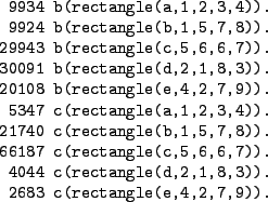
The counts produced by the MCMCMS run for the simple `six-hypothesis' prior and this `noisy' likelihood can be found in Fig 15. Recall that the `b' counts record the frequency with which hypotheses are proposed and the `c' counts record the frequency with which MCMCMS actually visited each hypothesis. The `b' counts in Fig 15 are similar to those found in Fig 10. This is as expected: rectangles are being proposed using the prior which is the same in both runs. Turning to the hypotheses actually visited, in Fig 10 only rectangles b and c are present (except for an initial visit to d) because only these two rectangles have non-zero likelihood. In contrast, in Fig 15 b and c have the highest frequencies, but the other rectangles are still visited: because the likelihood no longer rules them out entirely, they still have some posterior probability of being the `true' rectangle.

Figure 15: Counts from an MCMCMS run with with the tabular.slp prior and a `noisy' likelihood function (found in the file tutorial/out/noisy_concept_learning_out/tr_uc_rm_exs_tab_i100K__s1.counts).