A different prior

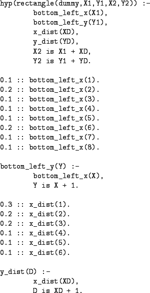
In the previous section there were only six hypotheses, so the use of MCMC was entirely unnecessary, except for tutorial purposes. In this section we start to move towards more realistic examples. Fig 11 shows an alternative prior over a hypothesis space of $8 \times 8 \times 6 \times 6 = 2304$ rectangles. Rectangles are sampled from this prior by first choosing the $X$ and $Y$ values for the bottom left corner of the rectangle, and then choosing the horizontal and vertical lengths of the rectangle. The definitions of x_dist/1 and y_dist/1 give a bias towards smaller rectangles. The definitions of bottom_left_x/1 and bottom_right_x/1 mean that $(2,3)$ and $(6,7)$ are a priori the most probable locations for the bottom left-hand corner. Note that now all rectangles get the same name: dummy. We keep this dummy argument in our representation of hypotheses to save us the bother of re-writing the likelihood functions. The code displayed in Fig 11 can be found in tutorial/slps/rects2304.slp.

Figure 11: An SLP for a simple prior over 2304 rectangles (found in the file tutorial/slps/rects2304.slp).

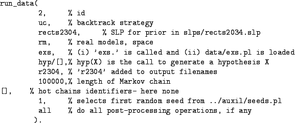
To use this new prior it suffices to have an appropriate run_data/11fact in the runs file. Fig 12 shows the relevant fact which can be found in tutorial/runs/concept_learning_run.pl. This is identical to the run_data/11fact shown in Fig 7, except that it points to a different file for locating the SLP prior (and uses a different id and output filename string).

Figure 12: Run information for using a more complex prior (found in the file tutorial/runs/concept_learning_run.pl).

Doing:
zcat tr_uc_rm_exs_r2304_i100K__s1.gz | grep '^c' | sort | uniq -c | sort -rn
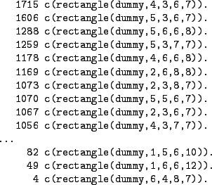
where tr_uc_rm_exs_r2304_i100K__s1.gz is the output file, gives us the frequency with which each rectangle was visited. Fig 13 shows that the most frequently visited rectangles (and hence those with highest estimated posterior probability) are as expected. They are consistent with the data and had high prior probability. However, the least visited rectangle rectangle(dummy,6,4,8,7) is not consistent with the data so it might seem odd that it was visited at all--after all it was visited 29 times which leads to an estimated posterior probability of $0.00029$ rather than the correct value of 0. What has happened is that, by chance, rectangle(dummy,6,4,8,7) is the initial model. For the first 28 iterations another inconsistent model was proposed, and the proposal is rejected. On the 29th iteration rectangle(dummy,3,4,9,8), a consistent rectangle, is eventually proposed. From that point on the chain visits only consistent models. Again, this shows the importance of discarding (for real applications) an initial `burn-in' part of the sample.

Figure 13: Highest and lowest counts using the more complex prior