Our first example is the `concept learning' problem illustrated in Fig 1. In concept learning the assumption is that there is an unknown target (or `true') concept which is simply a subset of some data space. Data consists of positive examples (examples in the target concept) and negative examples (examples outside the target concept). There is also a hypothesis space: sets which the learning system can hypothesise to be the true concept.
Consider a very simple concept learning scenario where the hypothesis
space contains a mere five hypotheses, each of which is a rectangle
(Fig 1). The data consists of two negative examples
(black dots in Fig 1) and a single positive example
(the white dot). Clearly, only the ![]() and
and ![]() rectangles are
consistent with the data.
rectangles are
consistent with the data.
In MCMCMS the user is required to define a prior over the hypothesis
space using an SLP. Fig 2 shows an SLP defining one
possible prior over our tiny hypothesis space. This SLP can be found
in tutorial/slps/tabular.slp. (This filename, and all others in this
section are given relative to the top level of MCMCMS once you have
unpacked it.)
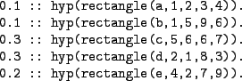 |
Each rectangle is represented by a term in first-order logic which gives the name of the rectangle and the co-ordinates of the bottom-left and top-right corners respectively. Hypotheses can be represented as the user sees fit: the important thing, as we shall see below, is to choose a representation that makes it easy to compute likelihoods.
A full explanation of how SLPs define probability distributions can be found, for example, in [CussensCussens2001]. In this simple example, each probability label in Fig 2 gives a prior probability for the corresponding rectangle. The choice of predicate symbol hyp/1 is arbitrary.
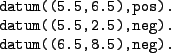
Similarly, the choice of data representation is a matter of
convenience, although using anything other than Prolog might involve a
lot of extra work. Fig 3 shows how we have chosen to
represent the three data points of Fig 1: we just
give co-ordinates and the class for each datapoint. This data can be
found in tutorial/data/exs.pl
 |
Now that prior and data have been determined we need to consider the
likelihood function. To see what sort of likelihood function needs to
be defined, consider the form of Bayes theorem relevant to concept
learning. Each datapoint ![]() is of the form
is of the form ![]() , where
, where
![]() is the datapoint's position and
is the datapoint's position and ![]() is its class. A
hypothesis
is its class. A
hypothesis ![]() is only required to predict an example's class given
its position. It need not make any predictions concerning positions.
(In statistical parlance, the co-ordinates giving the position of the
example are called either explanatory variables,
predictor variables or covariates.) Let
is only required to predict an example's class given
its position. It need not make any predictions concerning positions.
(In statistical parlance, the co-ordinates giving the position of the
example are called either explanatory variables,
predictor variables or covariates.) Let ![]() and
and ![]() represent the vectors of positions and classes of examples,
respectively. In the current case this means that
represent the vectors of positions and classes of examples,
respectively. In the current case this means that
![]() and
and
![]() . The
posterior
. The
posterior ![]() for any hypothesis
for any hypothesis ![]() can then be calculated as
follows:
can then be calculated as
follows:
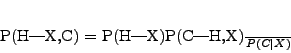 |
(1) |
| (2) |
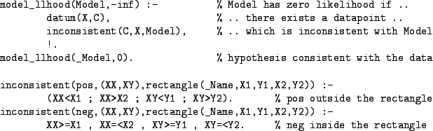
Code for computing likelihoods (in fact, log-likelihoods) is shown in
Fig 4. The first clause of predicate
model_llhood/2 declares that a Model (i.e. a
hypothesis) has log-likelihood ![]() (i.e. likelihood 0) if there
exists an example (X,C) which is inconsistent with the
model. If there are no inconsistent examples, then a log-likelihood of
0 (i.e. a likelihood of 1) is returned by the second clause. Note the
use of a cut (!) to ensure that model_llhood/2 defines a
function. This code can be found in the file tutorial/simple_concept_learning.pl.
(i.e. likelihood 0) if there
exists an example (X,C) which is inconsistent with the
model. If there are no inconsistent examples, then a log-likelihood of
0 (i.e. a likelihood of 1) is returned by the second clause. Note the
use of a cut (!) to ensure that model_llhood/2 defines a
function. This code can be found in the file tutorial/simple_concept_learning.pl.
 |
The likelihood is the place where the representations of the hypothesis space and the data meet. What is essential is that the definition of model_llhood/2 is consistent with whatever hypothesis and data representations are chosen.
Since MCMCMS uses the Metropolis-Hastings algorithm it does not
require the log-likelihoods directly. All that is needed is that,
given any two hypotheses ![]() and
and ![]() , the likelihood ratio is
computed. In our current example this ratio is simply
, the likelihood ratio is
computed. In our current example this ratio is simply
![]() . In some cases it is possible to compute
this ratio without going to the trouble of computing the individual
likelihoods (or log-likelihoods). However, in our current case there
is no such cleverness, we compute the ratio by computing
log-likelihoods and then computing the likelihood ratio. The code for
doing this is in Fig 5 and can be found in
tutorial/simple_concept_learning.pl. Note that LLi is instantiated at the
time lhood_canonical/5 is called, so
lhood_canonical/5 only needs to compute LLst, the
log-likelihood of MSt, to get the likelihood ratio.
. In some cases it is possible to compute
this ratio without going to the trouble of computing the individual
likelihoods (or log-likelihoods). However, in our current case there
is no such cleverness, we compute the ratio by computing
log-likelihoods and then computing the likelihood ratio. The code for
doing this is in Fig 5 and can be found in
tutorial/simple_concept_learning.pl. Note that LLi is instantiated at the
time lhood_canonical/5 is called, so
lhood_canonical/5 only needs to compute LLst, the
log-likelihood of MSt, to get the likelihood ratio.
 |
To run MCMCMS, both model_llhood/2 and lhood_canonical/5 must be defined by the user. However, if lhood_canonical/5 does not use model_llhood/2 then the latter can be given a `dummy' definition. See Section 7.1 for further details.
Now that prior, data and likelihood have been defined we can run MCMCMS to produce a sample from the posterior. To do this we start up Prolog (either Sicstus or Yap) and load the file tutorial/simple_concept_learning.pl which is displayed in Fig 6.
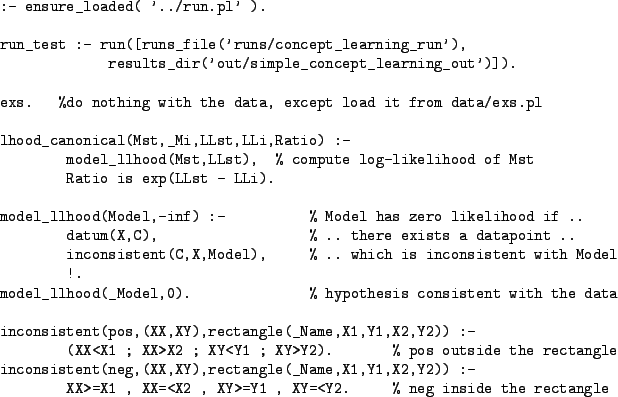 |
Most of the code in tutorial/simple_concept_learning.plconcerns the likelihood and has already been discussed. As for the rest, the first line loads in the main MCMCMS file ../run.pl. The predicate run_test/0 is there just to abbreviate the given call to the run/1 predicate. run/1 is a MCMCMS predicate (i.e. the user does not define it). The user calls run/1 with a list of options to perform a given MCMC run. These options are described in detail in Appendix A. In this case we just supply a runs_file and specify a directory for output.
A runs_file should be a Prolog file which defines a predicate run_data/11which sets parameters for a number of runs of the system. Fig 7 shows the run_data/11code relevant to our current example. This code can be found in tutorial/runs/concept_learning_run.pl. Detailed documentation for run_data/11can be found in Appendix B. The code given in Fig 7 says that the prior is defined in the file tutorial/slps/tabular.slp, where the slps directory is relative to the `main' file for running MCMCMS, that the predicate hyp/1 defines the prior, that data is in data/exs.pl (again data is relative to the main file) and that the run should be for 100000 iterations.
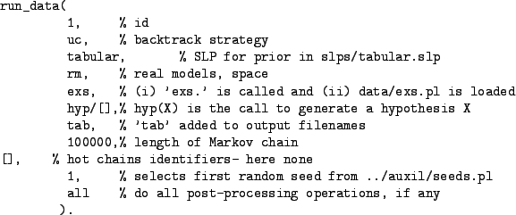 |
The rm parameter instructs that only `real' models should be considered. Whenever a failure is encountered, Prolog's backtracking is used to find the nearest model. Alternatively to this space, when fm is used, failures are reported at the top level of the MCMC and the algorithm registers a non-jump iteration. For an example illustrating the differences between rm and fm see [Angelopoulos CussensAngelopoulos Cussens2004, p.5].
The exs parameter plays a dual role. Firstly, this parameter determines the name of a file to load. Unless this file name is null, it is an error if the file does not exist or is not readable. This file will generally contain the data (it does in our current example), although this is not mandatory. As long as lhood_canonical/5 is defined to give the correct likelihood ratios, MCMCMS does not mind how the data is found. Secondly, the goal exs is called. This is a `hook' which can be used to do e.g. data pre-processing. As can be seen from Fig 6, in this case exs is defined to do nothing. If exs/0 were not defined the program would still run, but a warning would be generated.
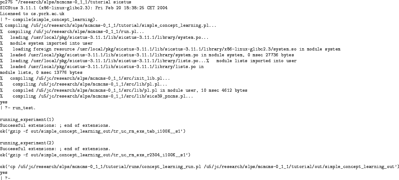
Once tutorial/simple_concept_learning.pl has been compiled, we kick off the run by simply entering run_test. at the Prolog prompt. Once the call to run_test/0 has completed the data from the run can be found in tutorial/out/simple_concept_learning_out. Recall that out/simple_concept_learning_out was the subdirectory specified in the results_dir option given to run/1. Fig 8 shows what the MCMCMS run looks like. As Fig 8 indicates, the run/0 call actually performs two MCMC runs since there are two run_data/9 facts in tutorial/runs/concept_learning_run.pl. The second experiment will be discussed in Section 2.2.
The models (in this case rectangles) visited during the MCMC run are
saved in the file tr_uc_rm_exs_tab_i100K__s1.gz. Note that the
filename is constructed from the various options defined using
run_data/11. This file is simply a (gzipped) text-file trace
of the models visited and so is 200001 lines long. (There is one extra
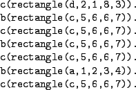
initial line to record the initial model.) In the trace file lines
starting with a `b' indicate proposed models and those with a `c'
indicate the current model.
Fig 9 shows the start of the trace file which we produced for this MCMCMS run. Rectangle d is the initial model (it is chosen using the prior). Rectangle c is then proposed and as the third line shows it is accepted and thus becomes the current model. Rectangle a is then proposed but the proposal is not accepted, so rectangle c remains the current model. In fact, inspection of the trace shows that the chain remains stuck at rectangle c until the 22nd iteration.
 |
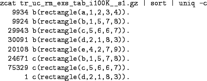
In this current tiny example it is trivial to pull out a simple
posterior from the trace. Fig 10 shows how to pull out
all the counts in the trace file. The last three lines of
Fig 10 show the models actually visited (as opposed to
merely proposed). The posterior probabilities estimated from the
trace for rectangles b and c are 0.248 and 0.752,
respectively, close to the correct values of 0.25 and 0.75. Note that
d gets an estimated posterior of
![]() . By chance it happened to be the initial model. A small
burn-in (throwing away an early part of the trace) would be enough to
delete it entirely. The first five `b' lines of Fig 10
show that models (rectangles) are being proposed according to the
prior distribution.
. By chance it happened to be the initial model. A small
burn-in (throwing away an early part of the trace) would be enough to
delete it entirely. The first five `b' lines of Fig 10
show that models (rectangles) are being proposed according to the
prior distribution.
![\includegraphics[width=0.9\textwidth]{exs.eps}](img4.png)